Meta-CLustering Algorithm (MCLA)

In this subsection, we introduce the third algorithm to solve the cluster ensemble problem. The Meta-CLustering Algorithm (MCLA) is based on clustering clusters. It also yields object-wise confidence estimates of cluster membership.

We represented each cluster by a hyperedge. The idea in MCLA is to group and collapse related hyperedges and assign each object to the collapsed hyperedge in which it participates most strongly. The hyperedges that are considered related for the purpose of collapsing are determined by a graph-based clustering of hyperedges. We refer to each cluster of hyperedges as a meta-cluster $\mathcal{C}^{(\mathrm{M})}$. Collapsing reduces the number of hyperedges from $\sum_{q = 1}^r k^{(q)}$ to $k$. The detailed steps are:

Construct Meta-graph.

Let us view all the $\sum_{q = 1}^r k^{(q)}$ indicator vectors $\mathbf{h}$ (the hyperedges of $\mathbf{H}$) as vertices of another regular undirected graph, the meta-graph. The edge weights are proportional to the similarity between vertices. A suitable similarity measure here is the binary Jaccard measure, since it is the ratio of the intersection to the union of the sets of objects corresponding to the two hyperedges. Formally, the edge weight $w_{a,b}$ between two vertices $h_a$ and $h_b$ as defined by the binary Jaccard measure of the corresponding indicator vectors $\mathbf{h}_a$ and $\mathbf{h}_b$ is: $w_{a,b} = \frac{\mathbf{h}_a^{\dagger} \mathbf{h}_b} { \Vert \mathbf{h}_a \Vert _2^2 + \Vert \mathbf{h}_b \Vert _2^2 - \mathbf{h}_a^{\dagger} \mathbf{h}_b}$.

Since the clusters are non-overlapping (e.g., hard), there are no edges amongst vertices of the same clustering $\mathbf{H}^{(q)}$ and, thus, the meta-graph is $r$-partite, as shown in figure 5.5.

Cluster Hyperedges.

Find matching labels by partitioning the meta-graph into $k$ balanced meta-clusters. Each vertex is weighted proportional to the size of the corresponding cluster. Balancing ensures that the sum of vertex-weights is approximately the same in each meta-cluster. We use the graph partitioning package METIS in this step. This results in a clustering of the $\mathbf{h}$ vectors. Since each vertex in the meta-graph represents a distinct cluster label, a meta-cluster represents a group of corresponding labels.

Collapse Meta-clusters.

For each of the $k$ meta-clusters, we collapse the hyperedges into a single meta-hyperedge. Each meta-hyperedge has an association vector which contains an entry for each object describing its level of association with the corresponding meta-cluster. The level is computed by averaging all indicator vectors $\mathbf{h}$ of a particular meta-cluster.^5.5 An entry of 0 or 1 indicates the weakest or strongest association, respectively.

Compete for Objects.

In this step, each object is assigned to its most associated meta-cluster: Specifically, an object is assigned to the meta-cluster with the highest entry in the association vector. Ties are broken randomly. The confidence of an assignment is reflected by the winner's share of association (ratio of the winner's association to the sum of all other associations). Note that not every meta-cluster can be guaranteed to win at least one object. Thus, there are at most $k$ labels in the final combined clustering $\mathbf{\lambda}$.

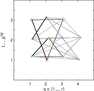
Figure 5.5 illustrates meta-clustering for the example given in table 5.1 where $r=4$, $k=3$, $k^{(1,\ldots,3)}=3$, and $k^{(4)}=2$. Figure 5.5 shows the original 4-partite meta-graph. The three meta-clusters are shown in red / $\circ$, blue / $\times$, and green / $+$. Consider the first meta-cluster, $\mathcal{C}_1^{(\mathrm{M})} = \{h_3, h_4, h_9\}$ (the red/$\circ$ markers in figure 5.5). Collapsing the hyperedges yields the object-weighted meta-hyperedge $h_{1}^{(\mathrm{M})} = \{v_5, v_6, v_7\}$ with association vector $(0,0,0,0,1/3,1,1)^{\dagger}$. Subsequently, meta-cluster $\mathcal{C}_1^{(\mathrm{M})}$ will win the competition for vertices/objects $v_6$ and $v_7$, and thus represent the cluster $\mathcal{C}_1 = \{ x_6, x_7\}$ in the resulting integrated clustering. Our proposed meta-clustering algorithm robustly outputs $(2, 2, 2, 3, 3, 1, 1)^{\dagger}$, one of the 6 optimal clusterings which is equivalent to clusterings $\mathbf{\lambda}^{(1)}$ and $\mathbf{\lambda}^{(2)}$. The uncertainty about some objects is reflected in the confidences 3/4, 1, 2/3, 1, 1/2, 1, and 1 for objects 1 through 7, respectively.

Figure 5.5: Illustration of Meta-CLustering Algorithm (MCLA) for the cluster ensemble example problem given in table 5.1. The 4-partite meta-graph is shown. Edge darkness increases with edge weight. The vertex positions are slightly perturbed to expose otherwise occluded edges. The three meta-clusters are shown in red / $\circ$, blue / $\times$, and green / $+$.